My readability metric found pockets in a sealed scroll. They were shredded.
I tried to read the best-looking pocket from my PHerc1203 readability atlas. It did not work.
That is the short version. The more useful version is why it did not work.
PHerc1203 is a sealed Herculaneum scroll listed among the First Letters volumes. The public list links its 9.362 µm volume, while this work used the newer 2.403 µm scan, so that specific scan’s prize eligibility remains unconfirmed. Prize status aside, its resolution made it a natural target for a simple technical question: can a CPU-only pipeline identify places inside a sealed scroll that look locally readable?
In my previous post, the PHerc1203 readability atlas, I described the metric. For each surface column, I sample a 62-layer depth window along the local normal. A location is marked “readable-class” if two things are true: occupancy is at most 0.5, and band-prominence is at least 0.55. In plain terms: is there enough dark space around the papyrus, and is there a strong enough bright band to suggest a surface?
The atlas found pockets that passed this test. The best one scored 0.89, comparable on my metric to PHerc1667, a scroll that has already been read. That was exciting enough to justify the next step, but not enough to claim anything. A local readability cue is not a readable surface. So I tried to turn the best pocket into an actual sheet.
It failed.
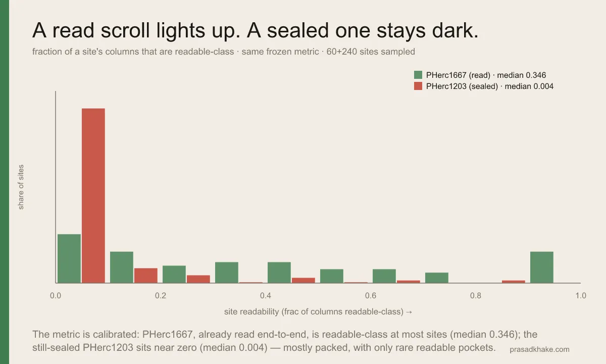
The atlas from the previous post: PHerc1203 (red) is mostly packed, with a thin tail of high-scoring “readable-class” pockets. This post is about what happened when I tried to read the best of those pockets.
The first failure: my own sheet-grower stalled
My first attempt was local and simple: my own sheet-growing code, starting from the high-scoring pocket. It worked on flat sheets — it could follow a surface when the geometry was cooperative. But PHerc1203 was not cooperative. The grower stalled on curvature.
The reason was straightforward: the method had no second-order depth prediction. It could follow a sheet while the surface stayed locally simple, but once the surface bent or changed depth in a more complicated way, the search lost the continuation. That did not prove the pocket was bad. It mostly proved my tracer was not good enough. So I moved to a stronger tool.
The second failure: Volume Cartographer grew away
The next test used Villa’s Volume Cartographer, the community-standard tracing tool. I seeded it at my best pocket, using the public m7 surface-prediction volume. This matters: the point was not to ask my metric whether the pocket looked good — it was to ask a separate surface-prediction system whether a coherent surface could be grown from there.
Volume Cartographer did grow a real surface — 33 cm² of it. But it grew away from my pocket. Only about 36 of 125,000 surface points landed near the pocket I had selected, and where it did touch the pocket, the result scored failed-class against the raw CT. I tried three independent configurations. They agreed.
That changed the shape of the problem. My metric said the pocket had a strong local readability signal. Volume Cartographer’s surface-prediction model saw no coherent surface there. Both statements can be true. The question became: what exactly was my metric responding to?
Two tests I had to retract
At this point I tried to build ceiling tests — ways to ask whether the pocket might still contain readable structure even if tracing failed. Both turned out to be invalid. I am including them because the retractions are part of the result.
The first was a single-peak-fraction test: check whether the depth profile has one dominant papyrus peak rather than several. A cleaner single peak should, in theory, be better. But the test failed its own calibration. The known-readable PHerc1667 scored 0.14; my PHerc1203 pocket scored 0.42. Higher was supposed to be better — and a valid readability metric cannot rank the already-readable scroll below the sealed pocket I was failing to trace. The failure mode was clear: papyrus fiber texture was being counted as false extra peaks. The test measured the wrong thing. I scrapped it rather than let it stand.
The second was a contiguous-area test. I measured about 0.8 mm² of candidate area and initially treated that as a hard ceiling. That was not valid either: my analysis block was 512³ voxels, about 1.23 mm wide. Even a modest 5 mm by 5 mm diagnostic region would exceed it, and the First Letters requirement is larger still: one connected 4 cm² region. The 0.8 mm² was block-truncated: a lower bound, not a conclusion.
The decisive test: raw CT at reading resolution
Two failed attempts and two invalid ceiling tests. That left the simplest test: stop inventing metrics and look at the data.
I fetched raw CT slabs around all top-13 pockets and inspected them at 2.4 µm — the resolution where reading happens. This was decisive because it did not depend on my metric, or any proxy score. It asked the direct visual question: are these pockets continuous wound sheets, or something else?
The answer was clear.
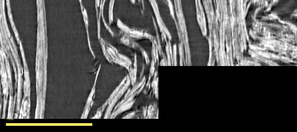
The best-scoring pocket, at reading resolution. This is not a continuous wound sheet — it is torn, frayed papyrus: swirling tangled fibers with voids. The metric fired here because a local depth window still catches one bright band with dark gaps. But there is no coherent surface to read.
Eleven of the thirteen top pockets are torn, tangled, shredded papyrus — swirling frayed fibers and voids, not continuous wound sheets. The other two came back thin or empty, also consistent with fragments. Zero of the thirteen showed a clean continuous readable sheet. The three highest-scoring pockets were all torn.
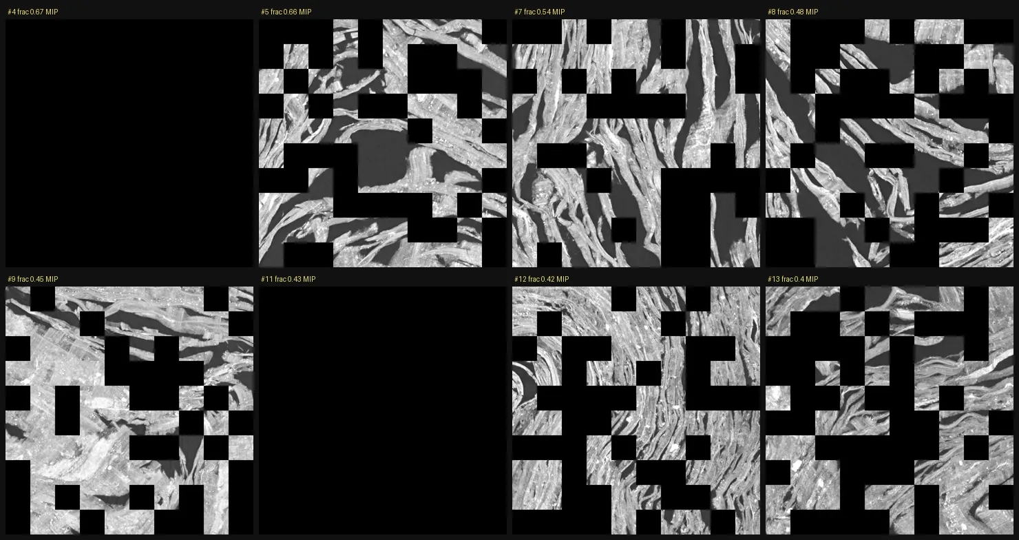
More of the top pockets at reading resolution (max-intensity projections). Every one is chaotic, torn, swirled — none is a flat continuous sheet. The black checkerboard is masked exterior. This is the negative result: my atlas’s best pockets were fragments, not hidden readable sheets.
What the metric actually found
The important finding is not “PHerc1203 is unreadable.” I do not know that, and this experiment does not show it. The finding is narrower:
Depth-occupancy readability is a local cue that torn fragments can pass.
A 62-layer window can catch one bright band with dark gaps around it — exactly what the metric rewards. But a torn papyrus fragment produces the same local signature as a small part of a good sheet. The metric does not know whether the band belongs to a continuous manifold, whether the surface extends into a segmentable sheet, or whether neighboring columns preserve a coherent geometry.
That explains the debugging trail. My metric fired because torn fragments can look locally readable. Volume Cartographer grew away because its surface-prediction model did not follow a coherent surface through the selected pocket. The single-peak test broke because torn structure and fiber texture defeat naive peak counting. Local separability remains a useful favorable cue under this pipeline, but it does not guarantee a readable surface.
What this does not prove
This part matters.
This does not show that PHerc1203 is unreadable. It does not show that nobody can read it. It does not show the scroll lacks readable regions. It shows that my occupancy-first atlas is biased toward torn fragments, and that my top-ranked pockets were not good read targets.
That means the genuinely readable regions, if they exist, may be exactly where my metric ranked low. A region that is densely packed and geometrically continuous — hard to separate locally — might score poorly on my metric while still being a better target for expert segmentation or a stronger model. Better surface-prediction models, GPU pipelines, expert manual segmentation, and higher-resolution rescans could all change what is reachable.
My survey does suggest PHerc1203 is hard: the scroll appears mostly packed in the regions I inspected. But hard is not impossible, and in this domain the difference matters. The right conclusion is not “the famous sealed scroll cannot be read.” It is: my first-pass readability atlas found local signals, and the highest-scoring signals were not coherent sheets.
The second search: coherence-first
So I ran the experiment the story above only proposed.
I built a coherence-first proxy: the size of the largest connected sheet-like component. In practice, that meant estimating local sheet normals with a structure tensor, linking neighboring surface patches only when their normals agreed within 12 degrees and their heights were consistent, then counting the grid cells in the largest connected component. Because the implementation caps and subsamples candidate cells, the resulting mm²-like values are comparative proxy scores, not direct physical area measurements.
I calibrated it first on three known-readable PHerc1667 blocks and three torn PHerc1203 pockets from the occupancy-first search. PHerc1667 had a median proxy score of 4.3; the torn PHerc1203 pockets scored 0.56 — a 7.7× separation under the frozen test. This is a small, cross-scroll calibration, not broad validation. A simpler local-planarity metric did not even clear that bar: torn fibers are locally planar too, so it could not tell a readable sheet from a clean-looking shred. I scrapped it.
Then I surveyed 180 stratified sites. This found something different from the occupancy-first ranking: 24 sites had coherence proxy scores of at least 3, and the top five reached roughly 25–39, with dominance scores of 0.97–0.99 (one component dominated the three largest). That looked like progress, but these values should be read as rankings, not measured sheet areas.
What the candidates actually were
The raw CT check changed the interpretation. I attempted to inspect the top eight coherence-ranked candidates. Seven produced usable occupancy measurements; all seven scored 0.61–1.0, against the local readable-class target of ≤0.5. Visually, they appeared as dense packed bundles: high mass, little empty space, and no reliable dark gutters between separable sheets. The highest-ranked site did not produce a usable occupancy measurement, so I exclude it from that conclusion.
So coherence-first exposed a different failure mode. Occupancy-first prioritized locally separated regions, but the top candidates were torn. The seven successfully inspected coherence-first candidates were comparatively continuous but packed. The first ranking found gutters without sheet coherence; the second found sheet-like continuity without local separability. This suggests that a useful target should score well on both dimensions.
The trap
That is the stronger hypothesis suggested by the two searches: the candidate sets exposed opposite failure modes. Where the occupancy-first ranking found dark gutters, its top candidates were shredded. Where the coherence-first ranking found large connected components, the seven measurable candidates were densely packed. No paired correlation was computed across all 180 sites, so this is an observed selection tradeoff, not yet evidence of scroll-wide anti-correlation.
This does not prove PHerc1203 is unreadable. I sampled about 180 sites plus top candidates, still only a fraction of the scroll, and the metrics are proxies: coherence, occupancy, and visual CT verification. Better models, higher-resolution rescans, or expert segmentation could still find a region where coherence and separation co-occur.
But the “add sheet coherence” fix is no longer sufficient by itself. The real next experiment is a paired joint gate: coherent and separated, measured at the same locations. It may find co-occurring regions; it may return empty in the sampled set. Either outcome would be stronger than inferring a scroll-wide relationship from two separately ranked candidate groups.