The same Herculaneum scroll query can fetch 1.3× — or 176× too much data
There is no single best zarr chunk size for reading the Herculaneum scrolls. On one 384³ region of Scroll 1, re-chunked five ways and read three ways, the read amplification — bytes fetched over bytes you actually wanted — ranged from 1.3× to 176×. Same data. The only thing that changed was the chunk geometry and the access pattern. Which chunk size is “best” is entirely a function of how you read.
I went looking for this because the Vesuvius Challenge core team said, out loud, that they don’t have a settled answer. In their public Discord last week, someone asked why different datasets use different chunk sizes. The replies: “different things need different sizes sometimes,” and then, plainly, “I think we all have different opinions on the best chunk size.” That’s an open, measurable question beneath a $1M Grand Prize whose current path depends on scaling virtual unwrapping. Data movement is a real part of that problem. So I measured it, on a laptop.
The setup
The scrolls are stored as chunked, compressed 3D volumes (OME-Zarr) in an open bucket you can stream without downloading terabytes. I pulled one 384³ region of Scroll 1 once (56.6 MB, ~26 s over home internet on a 16 GB M3), then wrote it back out locally at five chunk layouts — 32³, 64³, 128³, 256³, and an anisotropic 16×256×256 — asserting the decoded bytes were identical across all five before timing anything. Re-chunking locally is deliberate: it isolates chunk geometry as the single variable and strips out network jitter, so the numbers are about the chunking, not my Wi-Fi.
Then I replayed the three access patterns real pipelines use:
- train — random 64³ patches, the way an nnU-Net-style segmentation model samples.
- slice — full axial z-planes, the way a viewer pans through the volume.
- trace — an overlapping sequential 32³ walk, the way surface tracing moves along a sheet.
The metric is read amplification: compressed bytes fetched divided by bytes requested. A chunk store can only hand you whole chunks, so if you ask for a thin slice out of fat cubes, you pay for the whole cubes.
The result
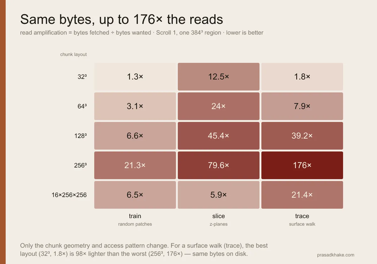
Read amplification for the same 384³ region of Scroll 1, re-chunked five ways and read three ways. The takeaway is the spread, not any single cell: getting chunk geometry wrong costs 10–100×, and the cheapest layout flips entirely with the access pattern — 32³ wins for training and tracing, the anisotropic 16×256×256 wins for slicing, and big 256³ cubes are a disaster for everything but bulk cubic reads.
| chunk | train | slice | trace |
|---|---|---|---|
| 32³ | 1.3× | 12.5× | 1.8× |
| 64³ | 3.1× | 24.0× | 7.9× |
| 128³ | 6.6× | 45.4× | 39.2× |
| 256³ | 21.3× | 79.6× | 176.0× |
| 16×256×256 | 6.5× | 5.9× | 21.4× |
Read down the columns and the story is clear. Big cubic chunks (256³) are a disaster for slice and trace access — 80× and 176× — because pulling one plane, or stepping along a surface, forces the store to ship whole stacked cubes you mostly throw away. The anisotropic 16×256×256 layout, shaped to match slice access, cuts slice amplification to 5.9× — about 13× better than 256³ — and is the best compromise among these five tested layouts when you do not know the access pattern in advance. It is still 5× worse than 32³ for training and about 12× worse for tracing. Small cubic chunks (32³) are best for random patch sampling and sequential tracing, at the cost of more, smaller requests.
None of these wins everywhere. That’s the whole point, and it’s exactly why the team’s answers differed: each person is optimizing for the pattern their tool uses, and each is locally right. The disagreement isn’t confusion — it’s the absence of a single optimum, now with numbers on it.
The other half: the Python reader doesn’t cache
While measuring this I hit a second thing. The Python Volume that streams these scrolls has no
chunk cache — read the same region twice and it fetches twice over the network. VC3D’s C++
readers cache; the Python path lost it when zarr 3 removed LRUStoreCache (the
use_volume_store_cache option in the tracer was deprecated for exactly this reason). Any
workload that revisits regions — training epochs, a viewer panning back, a tracer walking a
neighborhood — pays full network cost every time.
I put an opt-in LRU chunk cache back on Volume (villa #1177).
The same PR fixes a plain zarr-3 bug I tripped over first: Volume("Scroll1")[...] raises
TypeError on a multiscale group under the pinned zarr version (integer vs string member keys),
so remote multiscale reads are broken today regardless of caching.
How much the cache matters, measured over the real network against the production store (native 128³ chunks — the geometry the table above flags as expensive for slice and trace), from a laptop over home internet, cache off vs on:
| pattern | cache off (repeat) | cache on, repeat | speedup |
|---|---|---|---|
| random patches | 44.7 s | 0.028 s | 1618× |
| z-slices | 48.1 s | 0.071 s | 677× |
| sequential trace | 26.6 s | 0.025 s | 1045× |
Repeated access to a region collapses from tens of seconds to tens of milliseconds, because the
current Volume re-fetches over the network every time and the cache serves it from memory.
These are full realistic-pattern reads over the live link — a different, heavier measurement than
the PR’s own unit-scale microbenchmark (a small 32×64×64 repeat read, which shows ~300× because
both the fetch and the cached hit are tiny). At realistic patch and plane sizes on the production
128³ store, the gap widens to the hundreds-to-thousands. (Absolute seconds are inflated by a
home-internet link from India; both absolute time and the ratio will vary with network and hardware.
Even the first cached pass runs ~2× faster than uncached, because overlapping reads within one
pass share chunks.)
What this is good for
If you’re building on these volumes: pick chunk geometry to match your dominant access pattern, because the penalty for getting it wrong is 10–100×, not 10–20%. Slice-heavy viewer or ink-detection-over-planes work wants anisotropic, slice-friendly chunks. Random-patch training wants small cubes. And whatever you pick, cache repeat reads — it’s the one lever that helps every pattern at once.
This is the same method I’ve been applying to LLM inference — measure what actually moves across the memory hierarchy instead of arguing about it — pointed at a different problem. The harness, raw data, and re-chunking script are in the PR branch; the whole study reproduces on a laptop in a few minutes.
Caveats: one region, one machine, home internet. Local re-chunking isolates the chunk-size variable and removes network noise; amplification is the portable number and wall-times track it but vary with the link. Amplification is cold-cache except where the cache is stated.
Update (2026-08-05). The Vesuvius Challenge awarded villa PR #1177 — the Zarr 3 fix and chunk cache described above — a $1,000 July 2026 Progress Prize. More on what that means: My data-loader fix just won a $1,000 Vesuvius Challenge Progress Prize.